|
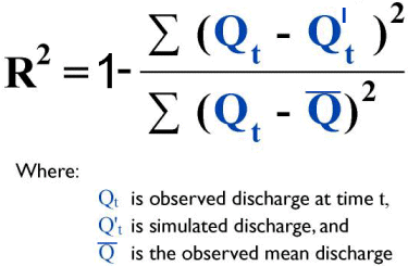
History and summary - Snowpack and snowmelt modelling - Water losses and routing - Operational experience and research extensions The HBV-model is a general-purpose hydrological model, named after the abbreviation of Hydrologiska Byråns Vattenbalansavdelning (Hydrological Bureau Waterbalance-section). This was the former section at SMHI, the Swedish Meteorological and Hydrological Institute, where the model was originally developed by Sten Bergström and colleagues. Its first application, to a 14 km² basin in northern Sweden, was described in Bergström (1972) and Bergström & Forsman (1973). The snow routine was added by Bergström (1975). A slightly modified version of HBV was used as the basis of the PULSE hydrochemistry model, which has been extensively used for investigations of surface water acidification and related issues (e.g. Bergström et al. 1985). The current operational version, HBV-96, is described in SMHI (1996) and its new features are outlined by Lindström et al. (in press).Like other general-purpose runoff models such as SHE, the US National Weather Service model (Anderson 1973), and the Canadian UBC model (Quick & Pipes 1977), HBV can handle both rainfall and snowfall and models the growth and decay of the snowpack. The normal time step in HBV is daily, though shorter time steps are available as an option and have been used in some applications (e.g. Hinzman & Kane 1991). The basin can be disaggregated into sub-basins, elevation zones, and land-cover types (forested, open, glacier, lake). Sub-basins may be connected in series (one basin draining into another) or parallel (draining separately to the outlet at which discharge is being predicted, e.g. when several separate basins feed a lake or hydropower reservoir). The purpose of the division into sub-basins is to allow for time lags in runoff from different parts of a large basin, or regional gradients in precipitation. Within a sub-basin runoff from each zone is added together so location does not matter. HBV and its variants have been applied in a wide range of countries and environments. Bergström (1992) mentions applications to over 200 basins in 30 countries, including nival and glacial basins in the Alps, Himalayas, New Zealand, Greenland and North America, arctic basins in Scandinavia and northern Alaska, and basins in both humid and semi-arid low-latitude environments such as Panama and Tunisia. Basins in which HBV has been applied range from <1 km² to 40 000 km². The predictive success of the model has generally been quantified by comparison of observed and simulated values of daily discharge using the standard Nash & Sutcliffe (1970) goodness of fit statistic:
R² increases from minus infinity towards one as the root-mean-square prediction error decreases towards zero. The percentage difference between observed and simulated mean or total discharge is also used. The treatment of the snowpack in HBV is based on a simple accounting algorithm whereby snow water equivalent increases when precipitation falls as snow, but decreases when snow melt takes place. The existence and amount of snowfall is predicted using meteorological input data extrapolated to the mean elevation of each sub-area of the basin. Parameters for this are the temperature lapse rate, rain/snow threshold temperature (not necessarily 0°C, and a ramp change between two temperatures is possible), and multipliers applied to measured precipitation to allow for underestimation of snowfall and any increase in precipitation with elevation. The existence and rate of snow melt in a sub-area is predicted from air temperature using the lapse rate, a critical temperature (which may be different from the threshold for snowfall), and a melt coefficient which is assumed to remain constant throughout the melt season. Allowance is made for the water holding capacity of the snowpack and for refreezing. Snow-covered area is not explicitly tracked but evidently falls in a stepped fashion over time during the melt season as progressively higher elevation zones lose their snow cover. It has been known for many years (e.g. Kuusisto 1980) that the best-fit degree-day melt factor for snow in a forested environment is smaller than for snow in open terrain, probably because of reduced near-ground wind speed and turbulent heat transfer. Recent versions of HBV allow a different melt factor to be specified for forested sub-areas and also for exposed glacier ice. The proportions of new rainfall or
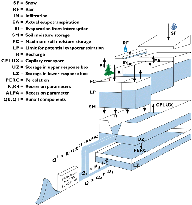
snowmelt which follow different pathways are determined by loss,
runoff, and routing algorithms shown schematically in the overall
system diagram (Figure 1). The key
controlling variable is the soil moisture content (SSM), which can
range from zero (dry soil) to some maximum (FC, the field capacity).
The potential evapotranspiration rate varies seasonally and is
specified using monthly values derived if possible from long-term
observations in or near the basin. The actual evapotranspiration rate
increases linearly from zero when the soil is dry to the potential
rate at some critical moisture content. It can be set to be higher in
forested zones and to reduce with altitude. The proportion of new
water contributing immediately to runoff increases nonlinearly with
soil moisture, as (SSM/FC). Thus the runoff percentage is zero when
the soil is dry, 100% when the soil is saturated, and the parameter
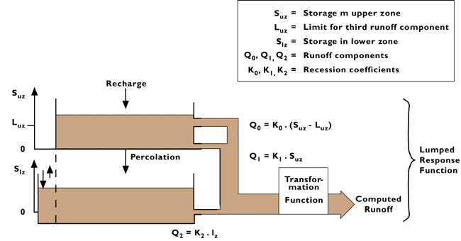
determines the shape of the curve between these limits. Figure 1. Structure of the HBV-96 model. Water not retained in the soil is routed through two stores, an upper one interpreted conceptually as saturated soil and a lower one representing groundwater. Water can percolate from the upper to the lower store, which has a slow linear outflow. In HBV-96 the upper store is nonlinear. In previous versions the store is linear until a second and faster outlet comes into operation above a specified level (Figure 2). PULSE uses a single store, but with three progressively faster overflow levels. Each variant of the model gives a nonlinear response to water input, with a dependence also on recent history through the initial level of soil moisture. Fast pathways operate only when the basin is already very wet, or becomes wet through a large input of rain or snowmelt. The number of adjustable parameters allows the model to be fitted to a wide range of basin conditions. The HBV-96 version has one parameter less and is easier to calibrate. The combined slow and fast outflow is
routed through a triangular filter. There is provision for channel
routing of runoff from tributary basins, using a modified Muskingum
method. Outflow from lakes is usually specified by a stage-discharge
rating curve but can be undamped or given by a lookup table to allow
for power station operating rules. Figure 2. Runoff routing in some earlier versions of HBV. The widespread use of HBV has generated considerable operational experience, and this has inevitably led to the recognition of difficulties in applying the model in particular situations. For example Vehviläinen (1986), working in Finland, and Hinzman & Kane (1991) working in a small Alaskan basin, found difficulty in correctly simulating the onset of significant meltwater discharge in basins in which the first meltwater is dammed for up to 3 days by snow or ice dams in river channels. Errors in simulating the start date of the spring melt are also mentioned by Andersson (1992) in a review of research done at SMHI on possible improvements to HBV and PULSE, and previously published only as Swedish-language reports. She notes that day to day errors in a model which gets the general seasonal pattern of runoff right could be through approximating the energy balance by a temperature index, particularly on cloud-free days with high radiation input and afternoon temperatures but low minimum temperature so that the mean temperature is low. A comparison using PULSE showed that an energy balance calculation using additional meteorological inputs was sensitive to wind speed and gave occasional bad errors within a slight overall improvement. Use of daily maximum and minimum temperatures gave a definite improvement on the standard method. However, a follow-up study using the same alternatives in HBV gave mixed results and Andersson concludes that a simple mean temperature is probably the most robust predictor to use, because it is spatially most stable. There is no special consideration of glaciers in the standard version of HBV apart from the possibility of using a higher melt coefficient, but it has been applied successfully to several glacial basins; for example, Bergström et al. (1982) obtained R2 = 0.83 for the Thjorsa basin in Iceland (2890 km2, 18% glacierised). Specific allowance for glaciers is made in a Swiss research version of the model, HBV3-ETH (Braun & Lang 1986). This has a seasonally variable degree-day coefficient to allow for dominantly radiation melt, with a multiplier to account for the albedo difference between ice and snow, and has been applied successfully to highly glacierised basins in Switzerland (Braun & Aellen 1990) and Nepal (Braun et al. 1993). The HBV-based model developed by Moore (1993) for use in a Canadian glacial basin is very similar, but as well as using a sinusoidal term in the melt equation also alters the runoff routing algorithm to allow for the seasonal evolution of the subglacial drainage system. Because HBV simulates the growth of the snowpack it is possible for model performance in the melt season to be imperfect not because of any problem with the snowmelt routine or the parameter values used in it, but because of incorrect simulation of snow accumulation. The threshold temperature for snowfall is a critical parameter in this respect. Several authors, including Vehviläinen (1986), have noted the desirability of independent evidence on snow cover and water equivalent. Bergström & Brandt (1985) showed that SWE could be mapped moderately well in open areas by airborne measurement of gamma-radiation attenuation by snow, but this is hard to distinguish from biomass attenuation in forested areas (Carroll & Carroll 1989). Braun & Aellen (1990) found glacier mass-balance measurements very useful in constraining the snow accumulation and melt parameters in HBV-ETH. Brandt (1991) used airborne radar to update the modelled snowpack, and Häggström (1994) compared simulated snow cover with AVHRR data. Ways to make greater use of satellite data in conjunction with HBV will be considered in a later phase of the HYDALP project. Non-standard applications of HBV and its variants include design flood estimation (Harlin & Kung 1992, using HBV) and scenario studies of the hydrological consequences of deforestation (Brandt et al. 1988) and climate change (Vehviläinen & Lohvansuu 1991, Braun et al. 1993, 1994). |


